Equal quantity is not always the least-risk choice
Continue with the specialty-flour purchase and related standard-flour futures. Suppose estimated price-change standard deviations over the hedge horizon are $3 per specialty bag and $2 per futures bag, with correlation 0.80. These are assumed estimates, not statistics inferred from our earlier two scenarios.
The bakery needs 100 specialty bags and each proxy futures contract represents 25 standard bags. We will choose the quantity of proxy exposure that minimizes modeled variance, then face the whole-contract constraint.
Predict the result, run the calculation, then make the requested change. Use signed numbers without units for numeric checks. Each calculation stands alone.
For decimal answers, round to two decimal places; trailing zeros are optional.
From five prices to a sample standard deviation
Here are five illustrative daily prices in dollars per bag. Subtract yesterday’s price from today’s: five price records give four paired daily changes, not five. Day 1 has no previous observation in this table.
| Day | Specialty spot price | Futures price | Spot change ΔS | Futures change ΔF |
|---|---|---|---|---|
| 1 | 30 | 22 | — | — |
| 2 | 25.50 | 21 | −4.50 | −1 |
| 3 | 27 | 20 | +1.50 | −1 |
| 4 | 28.50 | 19 | +1.50 | −1 |
| 5 | 30 | 22 | +1.50 | +3 |
Spot calculation:
- Mean change: (−4.50 + 1.50 + 1.50 + 1.50) / 4 = 0.
- Subtract the mean: −4.50, 1.50, 1.50, 1.50.
- Square and sum: 20.25 + 2.25 + 2.25 + 2.25 = 27.
- Sample variance: 27 / (4 − 1) = 9.
- Sample standard deviation: √9 = $3 per bag.
Futures calculation: mean change = 0; squared deviations sum to 1 + 1 + 1 + 9 = 12. Sample variance = 12 / 3 = 4; sample standard deviation = √4 = $2 per bag.
We divide by n − 1 = 3 because we are estimating a population variance from a sample of n = 4 changes. Variance has units (dollars per bag) squared; taking the square root restores dollars per bag. Two changes (three prices) are the mathematical minimum for this sample calculation. Four changes demonstrate the method but give a very uncertain estimate.
These are daily changes, so they estimate daily variability. For a different hedge horizon, use paired changes over that horizon. This constructed table reproduces the standard deviations 3 and 2. Its correlation is 1/3, not 0.80; the exercises below continue to use the separately assumed correlation 0.80.
Run it with Jax4J
Run the spot calculation first to load Jax4J and import Tensors; the futures calculation reuses that import. diff(0) takes consecutive price differences along axis 0. std(0, 1, false) calculates their sample standard deviation: axis 0, correction 1 (divide by n − 1), and no retained axis. Plain std() instead uses the population divisor n. item() extracts the scalar result.
Minimum-variance hedge ratio formula
For positive correlation in this buyer example, h* = correlation × spot-change standard deviation / futures-change standard deviation. h* is futures units per physical unit; direction is long for this buyer. An owner hedging a planned sale would use shorts for the same positive relationship.
Target contracts = h* × physical quantity / contract size. Use absolute dollar-per-unit changes with this quantity formula, comparable units and a common horizon. Do not insert percentage-return volatilities without changing the sizing convention.
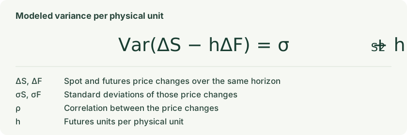
The variance is measured in (dollars per bag) squared, not dollars of profit.
A ratio above one can be appropriate when the proxy changes less per unit than the exposure. This differs from overhedging an exactly matching asset. Estimates, fees, daily-settlement financing, margin constraints and default are excluded; minimum variance does not mean a guaranteed outcome.
What does this mean in practice? Imagine a bakery that needs to buy flour. Higher flour prices make its purchase more expensive, but a long futures position can earn money to help cover that increase. The hedge ratio sets how much futures protection to buy; the contract-count formula turns that amount into actual contracts. Because flour and the futures contract may not move together perfectly, some uncertainty remains. Variance measures how widely the combined cost can fluctuate around its average: lower variance means a more predictable bill, not a guaranteed price. At the ideal hedge ratio, a correlation of 0.80 leaves 36% of the original variance (60% of the original standard deviation, or typical size of fluctuations). It does not mean every price increase or loss is reduced by 64%.
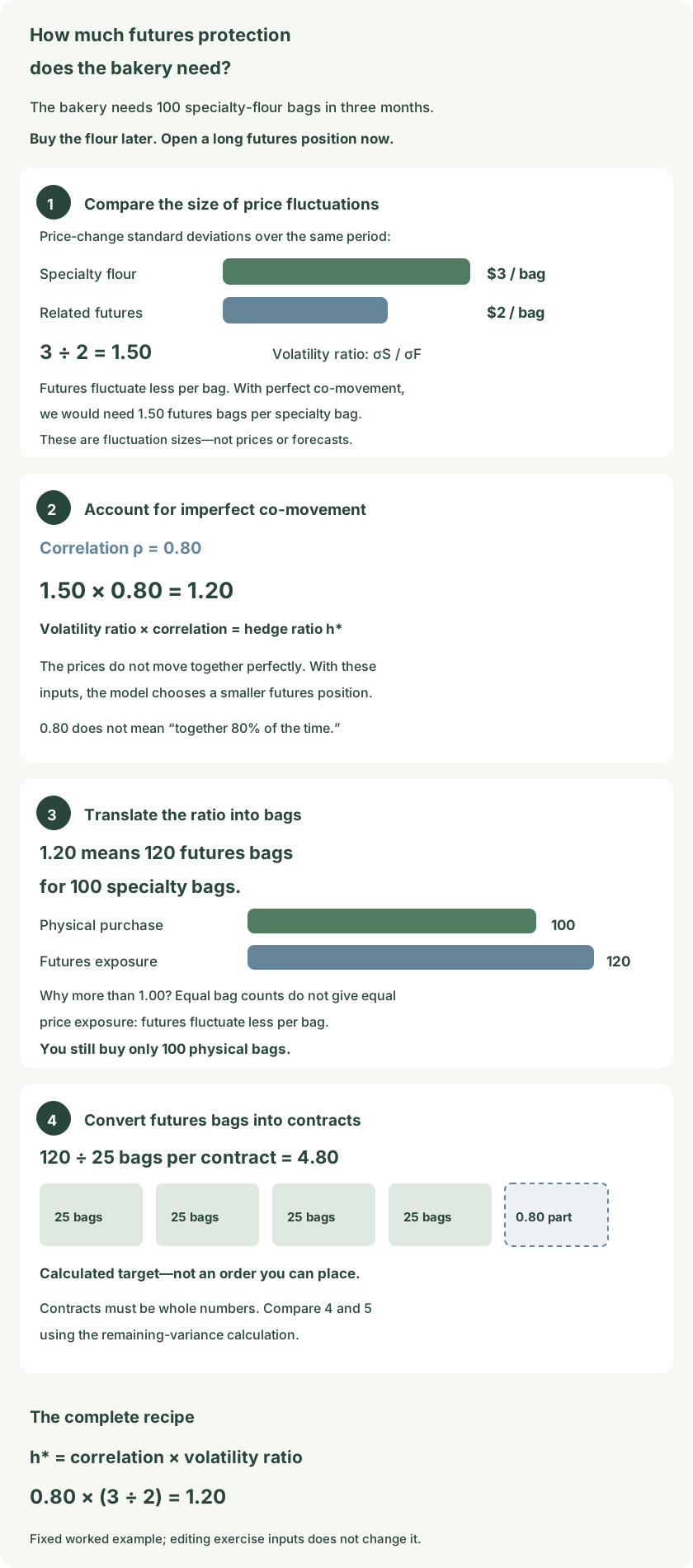
Exercise 1 — Compare change volatilities
Divide the $3 specialty-price-change standard deviation by the $2 futures-change standard deviation. These are measures of price changes over the same horizon, not the $30 and $22 price levels. The quotient describes relative movement size before correlation is included.
Exercise 2 — Include imperfect correlation
Multiply the volatility ratio by correlation 0.80. Then reduce correlation to 0.60 while leaving both standard deviations unchanged. With these fixed inputs, weaker co-movement reduces the model’s preferred proxy quantity.
Exercise 3 — Convert the original ratio into contracts
Restore correlation to 0.80. Multiply h* = 1.20 by the 100-bag physical exposure, then divide by 25 bags per proxy contract. This produces a continuous target before imposing the exchange’s whole-contract rule.
Read the picture
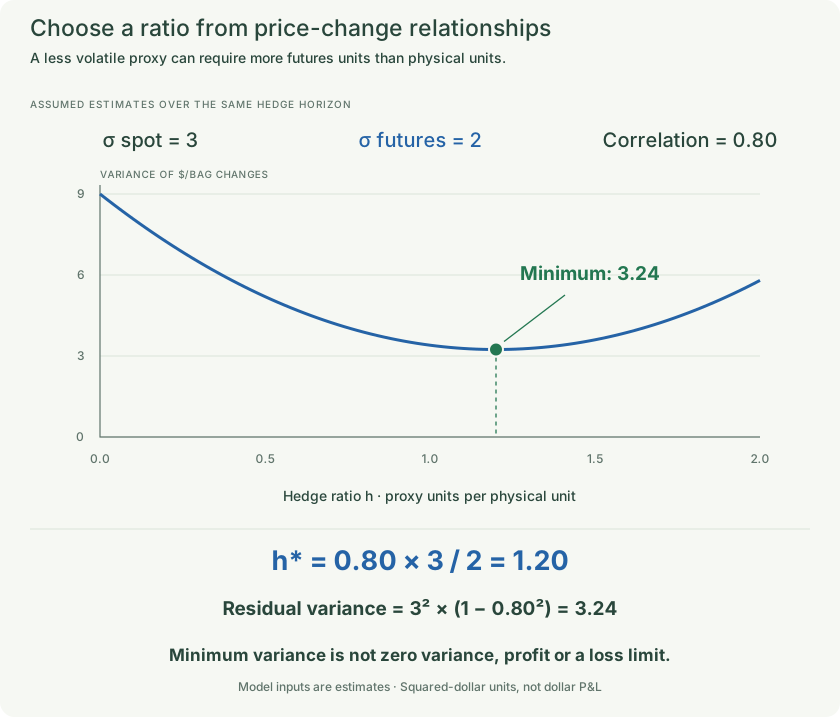
The diagram shows the stated worked example. Editing a calculation does not update the picture.
Exercise 4 — Find the ratio implied by whole contracts
Five proxy contracts represent 125 bags against a 100-bag physical need. Divide represented proxy quantity by actual physical quantity. Four contracts instead imply h = 1.00. These are the two nearby feasible hedge ratios.
Exercise 5 — Compare modeled variance after rounding
Use spot standard deviation 3, futures standard deviation 2 and correlation 0.80. The first line uses h = 1.00, the second h = 1.25. Compare the full variance expression rather than assuming that rounding up is always safer.
Exercise 6 — Measure the remaining variance
At the continuous optimum, residual variance is spot variance times one minus correlation squared. Start with correlation 0.80, then change both appearances to 0.60. The remaining fraction concerns variance, not the proportion of any single future loss.
Read the picture
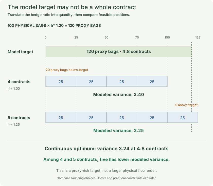
The diagram shows the stated worked example. Editing a calculation does not update the picture.
Exercise 7 — Interpret a ratio above one
Our h* is 1.20 because the related futures’ price changes are less volatile per bag. The hedge is still tied to the bakery’s need and an explicit risk model. Compare this with adding unmatched contracts merely because someone expects a price rise.
Remember
Estimate the relationship between changes over a common horizon, choose the ratio, then convert to whole contracts. Recheck risk after rounding. A minimum-variance model does not guarantee no loss or no margin call.