Bootstrap discount factors from market prices
Earlier lessons supplied a zero curve as an input. A trading desk instead sees prices of instruments with several cash flows and must infer a consistent curve. Start with the shortest instrument, solve one new discount factor at a time, and verify that the curve actually prices what was used to build it.
Predict the result, run the standalone calculation, then make any requested edit before answering. Each exercise retains its own stated inputs. Enter numeric answers without units and round to two decimals unless four are requested. Code is provided to explore the finance; no new Java syntax is required.
How does a bootstrap recover discount factors?
A bootstrap solves the shortest available maturity first and reuses known discount factors to isolate the next unknown. All instruments here belong to the same fictional certain-payment currency/discounting model; mixing sovereign, risky and differently collateralized prices without adjustments would break that assumption.
| Calibration instrument | Stated quote and dated cash flows |
|---|---|
| One-year deposit | Invest 100 now; receive 104 at year one |
| Two-year annual coupon bond | Price 99; receive 4 at year one and 104 at year two |
| Three-year annual coupon bond | Price 100; receive 5 at years one and two, and 105 at year three |
These factors are dimensionless. Prices are on coupon dates so no accrued-interest adjustment is needed in this simplified construction.
A useful curve must reprice each calibration instrument, not only generate smooth-looking rates. Retain precision in solved factors and inspect residuals in price units. In real data, bid/ask, noise and incompatible instruments may require a fitting objective instead of forcing exact equality.
For a point between known dates, this lesson stipulates linear interpolation of log discount factors. At 1.5 years, , so is their geometric mean. This keeps factors positive and implies a constant continuous forward rate between these two points; other interpolation rules produce different intermediate prices.
Do not extrapolate beyond the last calibrated maturity without another explicit assumption. A negative discount factor cannot price a certain positive future dollar in this model. A positive factor above one, or a rise between two dates, is not automatically invalid when negative interest rates are permitted.
Scenario and assumptions
Use one currency, annual coupons, certain payments, no fees/default/taxes and dates exactly at year boundaries. Deposit interest is 4% simple over its one-year term, giving the stated 104 repayment. Instruments have the same valuation basis. The 1.5-year factor is an interpolation assumption, not a separately observed quote. Each cell writes the prior solved factors algebraically so it can run independently without hidden notebook state.
Exercise 1 — Start with the single-payment instrument
A deposit exchanges 100 today for 104 in one year. The factor must turn 104 back into 100. Use floating-point division in the provided calculation. This is simpler than guessing a zero rate and then iterating toward a known price.
Exercise 2 — Isolate the next bond’s final payment
The two-year bond price is 99. Its first coupon is already worth . Remove that known present value, leaving the price of the final 104 payment. Divide by 104 to obtain . Do not apply the deposit’s rate unchanged for another year unless the data imply it.
Exercise 3 — Add the third maturity
The three-year bond costs 100 and pays 5, 5 and 105. Subtract the present values of the first two coupons using the already solved factors, then divide by the final 105. The year-three coupon is inside 105; do not omit it or subtract it twice.
Read the picture
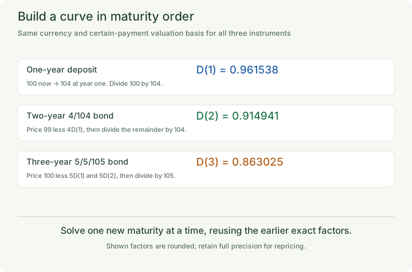
A one-year deposit gives ; coupon-bond prices then isolate and .
The illustration is a fixed worked example. Editing a calculation does not update it.
Exercise 4 — Measure the error from premature rounding
Suppose someone stores as 0.9615 and as 0.9149 rather than keeping their exact solved values. Reprice the two-year bond with those rounded factors and subtract its 99 input price. A two-decimal display can hide the residual, so report four decimals.
Exercise 5 — Interpolate a factor between observed maturities
At 1.5 years, use the midpoint of and . Exponentiating gives their geometric mean. The factor is positive and between its endpoints in this particular positive-rate example. Interpolating zero yields or discount factors directly would be a different assumption.
Exercise 6 — Rebuild when a calibration price changes
Price a certain 1,000 payment at 1.5 years using that interpolated factor. Run the baseline, then change the two-year bond’s price from 99 to 98 inside the expression. Keep the deposit quote fixed. This changes and the interpolated factor; a complete rebuilt curve would also recompute later .
Read the picture
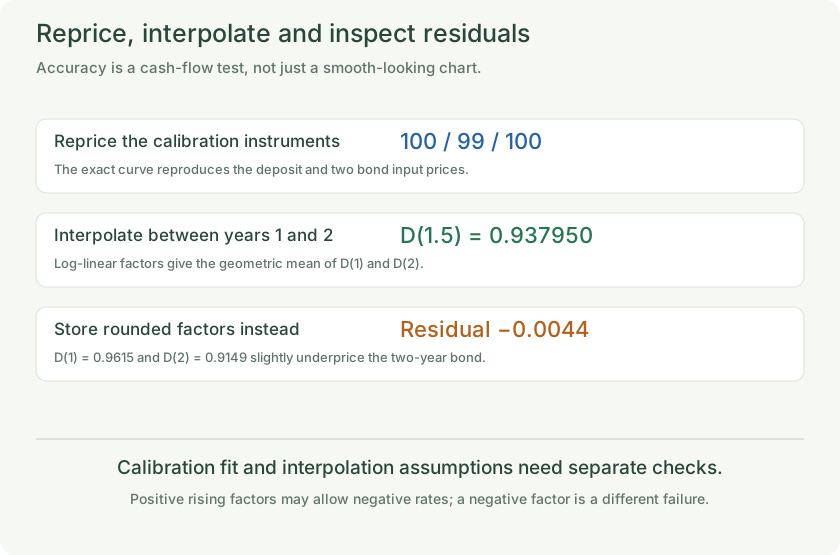
The exact curve reprices the deposit and both bonds; log-linear interpolation gives , while rounded factors leave a price residual.
The illustration is a fixed worked example. Editing a calculation does not update it.
Exercise 7 — Reject an impossible solved factor for this model
For a separate bad-input diagnostic, set the two-year bond price to just 3 while keeping its positive 4/104 cash flows and the same . Its first coupon alone is worth more than 3, leaving a negative implied . Distinguish this failure from a positive factor rising because of a negative forward rate.
Remember
Bootstrap known cash flows in maturity order and reprice every input. Keep full precision, declare interpolation and avoid silent extrapolation. Distinguish impossible negative discount factors from valid negative-rate behavior. A smooth curve is not enough if it cannot reproduce its calibration prices on a consistent valuation basis.