Convexity explains the error in duration
A straight line understates the curvature of a fixed-payment bond’s price. Use a five-year zero to isolate that curvature without a coupon schedule, and check rather than assume that adding a second term is accurate enough.
Predict, run the provided Java calculation, then make the requested edit before answering. Each exercise uses its own stated inputs. Enter numbers without units; round final answers to two decimals unless four are requested. Keep intermediate precision. Code supports the finance rather than teaching Java syntax.
How does convexity improve a price estimate?
For a fixed-payment bond discounted at one continuous yield , , , and . The continuous-yield approximation is
has year units; has year-squared units. Annual-yield convexity has a different formula; do not combine conventions.
A certain zero paying $1,000 at year five has , and . The exact shocked price is . Ordinary positive fixed cash flows give positive convexity here: the curve lies above its tangent. The positive second-order correction applies to upward and downward rate moves because is squared.
Define the residual as exact shocked price minus approximate shocked price. A smaller absolute residual is evidence of a better local approximation for that scenario, not proof it will work for any shock. Embedded exercise rights can change cash flows and effective convexity, including its sign.
Scenario and assumptions
All rates in this lesson compound continuously. Use a zero with five years remaining and no credit risk or embedded options. Base yield is 3%; ±200 bp shocks are illustrative stress scenarios. No coupon reinvestment occurs for this zero. Figures use fixed inputs.
Exercise 1 — Apply duration alone
A +200 bp move is . Estimate the new price with and no curvature term. The price estimate should fall.
Exercise 2 — Compute the exact benchmark
Reprice the same $1,000 payment at a continuous 5%. Keeping the maturity and cash amount fixed isolates the rate effect.
Exercise 3 — Calculate the curvature correction
Use . This is a positive dollar adjustment to the duration-only price, not an additional loss.
A tangent misses curvature
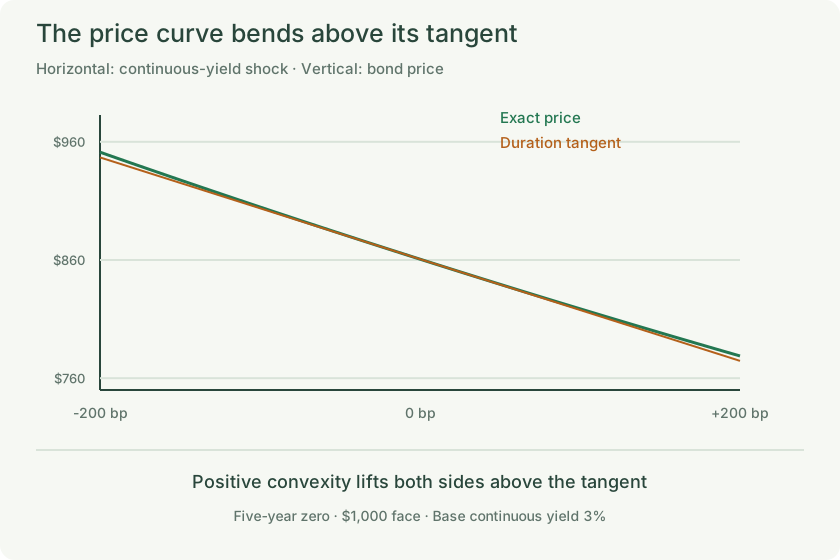
Base $860.71; +200 bp duration-only $774.64; second-order $778.94; exact $778.80.
The illustration uses fixed worked inputs. Editing code does not update it.
Exercise 4 — Combine both orders
Add the duration and convexity terms before rounding. This approximates a 9.5% decline rather than 10%.
Exercise 5 — Measure what the approximation misses
Subtract the unrounded second-order result from exact repricing. Retain the sign; a negative residual means the approximation is too high.
Exercise 6 — Reverse the rate shock
Run the positive shock, then change all three 0.02 inputs to -0.02. The base rate remains 3%; the stressed rate becomes 1%. The duration term reverses sign while convexity remains positive.
Opposite shocks are asymmetric
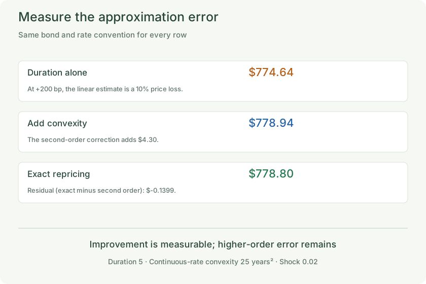
Exact gain at −200 bp: $90.52. Exact loss at +200 bp: $81.91. Convexity adds to both tangent estimates.
The illustration uses fixed worked inputs. Editing code does not update it.
Exercise 7 — Test a larger move and the fixed-cash-flow assumption
For +400 bp the code measures the exact-minus-second-order residual. Its absolute size is larger than for +200 bp. Also consider a callable bond whose issuer may redeem when rates fall.
Remember
Use a consistent compounding convention for duration and convexity. Square the rate move in the second-order term, retain full precision, and measure signed residuals against exact prices. Exercise rights and large shocks require more than a local expansion.